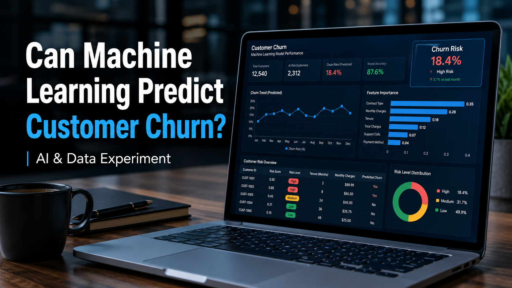
Can Machine Learning Predict Customer Churn?

Imagine a business with 10,000 customers. Some use the product every day. Others are becoming less active. Some are contacting customer support more often, while others have not logged in for weeks. The question is simple:

Can we identify which customers are at risk of leaving before they actually stop using the service? To explore this question, I created a small machine learning experiment. No complex architecture. No deep learning. No large-scale infrastructure. Just Python, Google Colab, synthetic data, and Logistic Regression.

What Did I Want to Test?

The goal of this experiment was not to build a production churn prediction system. I wanted to test something much simpler:

Can a simple machine learning model recognize customer behavior patterns associated with churn risk? Customer churn happens when a customer stops using a product or service. For example, a customer may cancel a subscription, stop using an internet service, or move to a competitor. Being able to identify customers who are likely to churn can help businesses prioritize retention efforts before those customers leave.

Creating the Experimental Dataset

Because this was an early-stage experiment, I used synthetic data. I generated approximately 5,000 customer records with several behavioral features:

tenure_months
monthly_spend
login_frequency
complaint_count
support_tickets
days_since_last_login

I then intentionally introduced several patterns into the dataset. Customers were designed to have a higher churn probability when they:

Longer inactivity      → Higher churn risk
More complaints        → Higher churn risk
More support tickets   → Higher churn risk

Other behaviors were designed to reduce churn probability:

Higher login frequency → Lower churn risk
Longer tenure          → Lower churn risk

I also intentionally included one variable that had no direct relationship with churn:

monthly_spend → no intentional relationship with churn

The idea was to see whether the model could distinguish meaningful predictive signals from a feature that was mostly irrelevant.

Defining the Synthetic Churn Pattern

Because this was a controlled experiment, I created the churn probability myself. The simplified logic looked like this:

risk_score = (
    (days_since_last_login * 0.07)
    + (complaint_count * 0.50)
    + (support_tickets * 0.25)
    - (login_frequency * 0.08)
    - (tenure_months * 0.02)
)

I then converted that score into a probability between 0 and 1.

churn_probability = 1 / (
    1 + np.exp(-(risk_score - 3))
)

This formula represents the ground truth of the synthetic experiment. Because I already know how the data was generated, I can later compare what the model learns with the relationships I intentionally created.

How Does the Model Learn?

For this experiment, I used LogisticRegression from scikit-learn. Despite the word regression in its name, Logistic Regression is commonly used for binary classification problems. In this case:

0 = Customer stays
1 = Customer churns

The features and target were separated like this:

X = df.drop(columns=["churn"])
y = df["churn"]

The dataset was then divided into training and testing data:

X_train, X_test, y_train, y_test = train_test_split(
    X,
    y,
    test_size=0.20,
    random_state=42,
    stratify=y
)

That gives us:

80% → Training Data
20% → Testing Data

The model was then trained using:

model = LogisticRegression(max_iter=2000)
model.fit(X_train, y_train)

The overall workflow is simple:

Customer Data
      ↓
Train/Test Split
      ↓
Logistic Regression
      ↓
Churn Probability
      ↓
Model Evaluation

Predicting Churn Probability

Instead of producing only a binary prediction such as:

CHURN
or
NOT CHURN

the model can estimate a probability. For example:

Customer A → Churn Risk: 12%
Customer B → Churn Risk: 51%
Customer C → Churn Risk: 89%

The probability can then be translated into a simple business risk level:

def get_risk_level(probability):
    if probability >= 0.70:
        return "HIGH"
    elif probability >= 0.40:
        return "MEDIUM"
    else:
        return "LOW"

Which creates:

0%  ───────── 40% ───────── 70% ───────── 100%
        LOW          MEDIUM          HIGH

In a real business scenario, these risk levels could support different actions:

LOW
→ Normal engagement

MEDIUM
→ Proactive engagement

HIGH
→ Retention campaign

Accuracy Is Not the Only Metric That Matters

One of the easiest mistakes in machine learning is focusing on a single number:

Accuracy

Suppose a model achieves:

Accuracy: 85%

That sounds good. But for customer churn, accuracy alone may not tell us whether the model is actually useful. Imagine that 100 customers are truly going to churn. If the model identifies only 60, then:

Detected churn customers : 60
Missed churn customers   : 40
Recall                   : 60%

That means 40% of the customers we wanted to identify were missed. Because of this, I evaluated the model using several metrics:

Accuracy
Precision
Recall
F1 Score
ROC-AUC

In Python:

accuracy = accuracy_score(y_test, y_pred)
precision = precision_score(y_test, y_pred)
recall = recall_score(y_test, y_pred)
f1 = f1_score(y_test, y_pred)
roc_auc = roc_auc_score(y_test, y_prob)

This leads to an important lesson:

The model with the highest accuracy is not always the model that creates the most business value. The most important metric depends on what decision the model is supposed to support.

Can the Model Recover the Signals We Created?

This was the most interesting part of the experiment. Because the dataset was synthetic, I already knew the expected relationships:

complaint_count
↑
churn risk ↑

days_since_last_login
↑
churn risk ↑

support_tickets
↑
churn risk ↑

login_frequency
↑
churn risk ↓

tenure_months
↑
churn risk ↓

And:

monthly_spend
→ intentionally irrelevant

After training the model, I inspected its coefficients:

feature_effect = pd.DataFrame({
    "feature": X.columns,
    "coefficient": model.coef_[0]
})
feature_effect["absolute_importance"] = (
    feature_effect["coefficient"].abs()
)

For Logistic Regression:

Positive coefficient
→ increases predicted churn probability

Negative coefficient
→ decreases predicted churn probability

Coefficient near zero
→ little predictive influence

If the model is behaving as expected, the learned direction should roughly match the ground truth used to generate the synthetic data. This is one of the advantages of a controlled synthetic experiment. We know the answer beforehand. So instead of asking only:

How high is the accuracy? We can also ask: Did the model actually learn the correct underlying signals?

Simulating a High-Risk Customer

I created a sample customer with the following profile:

high_risk_customer = {
    "tenure_months": 4,
    "monthly_spend": 750000,
    "login_frequency": 2,
    "complaint_count": 5,
    "support_tickets": 6,
    "days_since_last_login": 35
}

In human-readable form:

Tenure                 : 4 months
Login frequency        : Very low
Complaints             : High
Support tickets        : High
Days since last login  : 35 days

The model assigned this profile a high churn probability. I then simulated another profile:

improved_customer = {
    "tenure_months": 4,
    "monthly_spend": 750000,
    "login_frequency": 18,
    "complaint_count": 1,
    "support_tickets": 2,
    "days_since_last_login": 2
}

Now the profile looks like:

Login frequency        : Higher
Complaints             : Lower
Support tickets        : Lower
Days since last login  : More recent

The predicted churn probability decreases. This is useful for understanding how the model reacts to different input profiles. However, this creates an important question. If changing the customer profile lowers the model's predicted churn risk, does that mean those changes will cause the customer to stay? No.

Prediction Is Not Causation

Machine learning is very useful for answering questions such as:

Which customers have a higher probability of churn? But predictive models do not automatically answer: What causes customers to churn? Suppose the model finds:

Higher complaint count
        ↓
Higher predicted churn risk

We can reasonably say:

A higher complaint count is associated with higher churn risk in this dataset. But we should not immediately conclude:

More complaints
        ↓
CAUSE
        ↓
Customer churn

There may be another underlying factor. For example:

Poor service quality
      ↓
      ├── More complaints
      │
      └── Higher churn risk

In this case, complaints may be a signal rather than the true root cause. To investigate cause-and-effect relationships, we would need approaches such as:

Controlled experiments
A/B testing
Causal inference

Prediction and causation answer fundamentally different questions.

Limitations of This Experiment

There is one major limitation:

The dataset used in this experiment is synthetic. The customer behavior patterns were intentionally created for the experiment. Therefore, the results should not be interpreted as evidence that:

Complaints are the main cause of real-world churn.
Inactive customers will definitely leave.
This model is ready for production.

The experiment only demonstrates that:

A simple model such as Logistic Regression can learn churn-related patterns when predictive relationships exist in the data. In other words:

This experiment
      ≠
Production churn model

It is closer to:

Controlled ML Experiment
+
Proof of Concept
+
Learning Exercise

What Did I Learn?

Even from a simple experiment, several lessons stood out.

1. Simple Models Are Still Useful

Not every machine learning problem needs:

Deep Learning
Neural Networks
LLMs
Complex architectures

A simple LogisticRegression model can already provide a useful baseline.

2. Accuracy Should Not Be Viewed in Isolation

A model may have high accuracy while still missing the cases we actually care about. Depending on the use case:

Recall
Precision
F1
ROC-AUC

may provide more useful information.

3. Model Interpretability Matters

Looking at coefficients or feature importance helps answer:

What is the model actually learning? A high evaluation score without understanding model behavior can be misleading.

4. Prediction Is Different From Causation

A predictive relationship:

Feature X
   ↓
Higher churn probability

does not automatically mean:

Feature X
   ↓
CAUSES
   ↓
Customer churn

5. Machine Learning Is More Than Choosing an Algorithm

The algorithm is only one component. A useful ML workflow looks more like:

Problem
   ↓
Data
   ↓
Assumptions
   ↓
Model
   ↓
Evaluation
   ↓
Interpretation
   ↓
Business Decision

Understanding those relationships is often more important than simply choosing a more sophisticated model.

Next Experiment

The natural next step is to replace the synthetic dataset with a real-world customer churn dataset. That raises a much more interesting question:

Do the patterns found in a controlled synthetic experiment also appear in real customer data? After that, I want to compare:

Logistic Regression
        vs
Random Forest
        vs
Gradient Boosting

But instead of asking only:

Which model has the highest accuracy?

I think the more useful question is:

Does the added model complexity actually produce a meaningful improvement? For example:

Model                    ROC-AUC    Complexity
------------------------------------------------
Logistic Regression        ?          Low
Random Forest              ?          Medium
Gradient Boosting          ?          Higher

If a significantly more complex model only improves the result slightly, the simpler model may still be the better engineering choice. Because in the end:

A good machine learning model is not simply the model with the highest score. A good model is one that helps us make better decisions.